
seaborn으로 그래프 그리기
seaborn : 간편하게 근사한 그래프 생성
matplotlib : 원하는대로 커스텀하게 그래프 생성
사용 방법

일별 데이터로 자동으로 평균값을 구해 month로 그래프를 그려줌

디자인

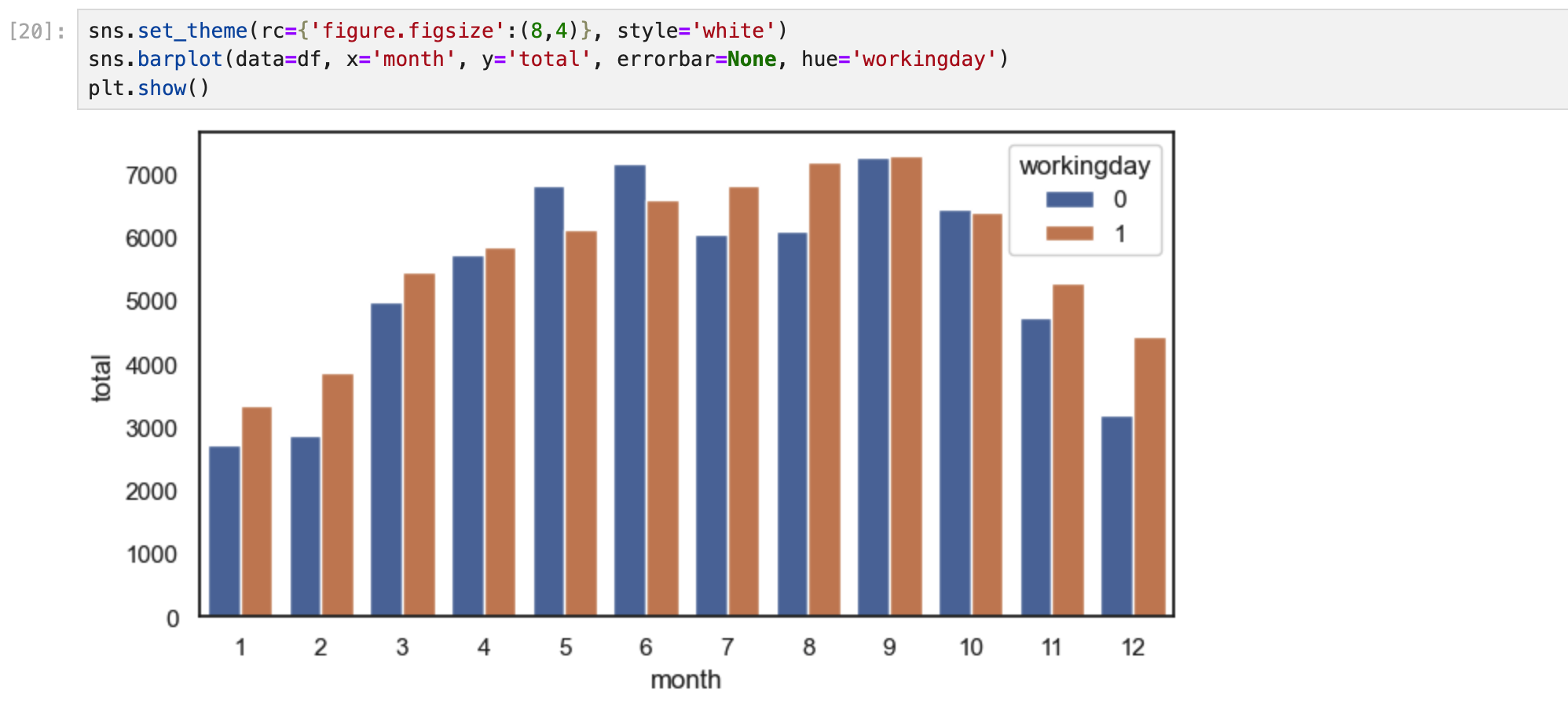
set_theme()함수로 그래프 커스터마이징하기


실습
import pandas as pd
import seaborn as sns
import matplotlib.pyplot as plt

bike_df = pd.read_csv('data/bike.csv')
sns.set_theme(rc={'figure.figsize': (10, 5)}, style='white')

# 여기에 코드를 작성하세요.
sns.barplot(data=bike_df, x='quarter', y='registered', errorbar=None, hue='workingday')
데이터 분포 시각화 1

stripplot

swarmplot
많이 분포된 곳은 나란히 옆으로 나오게
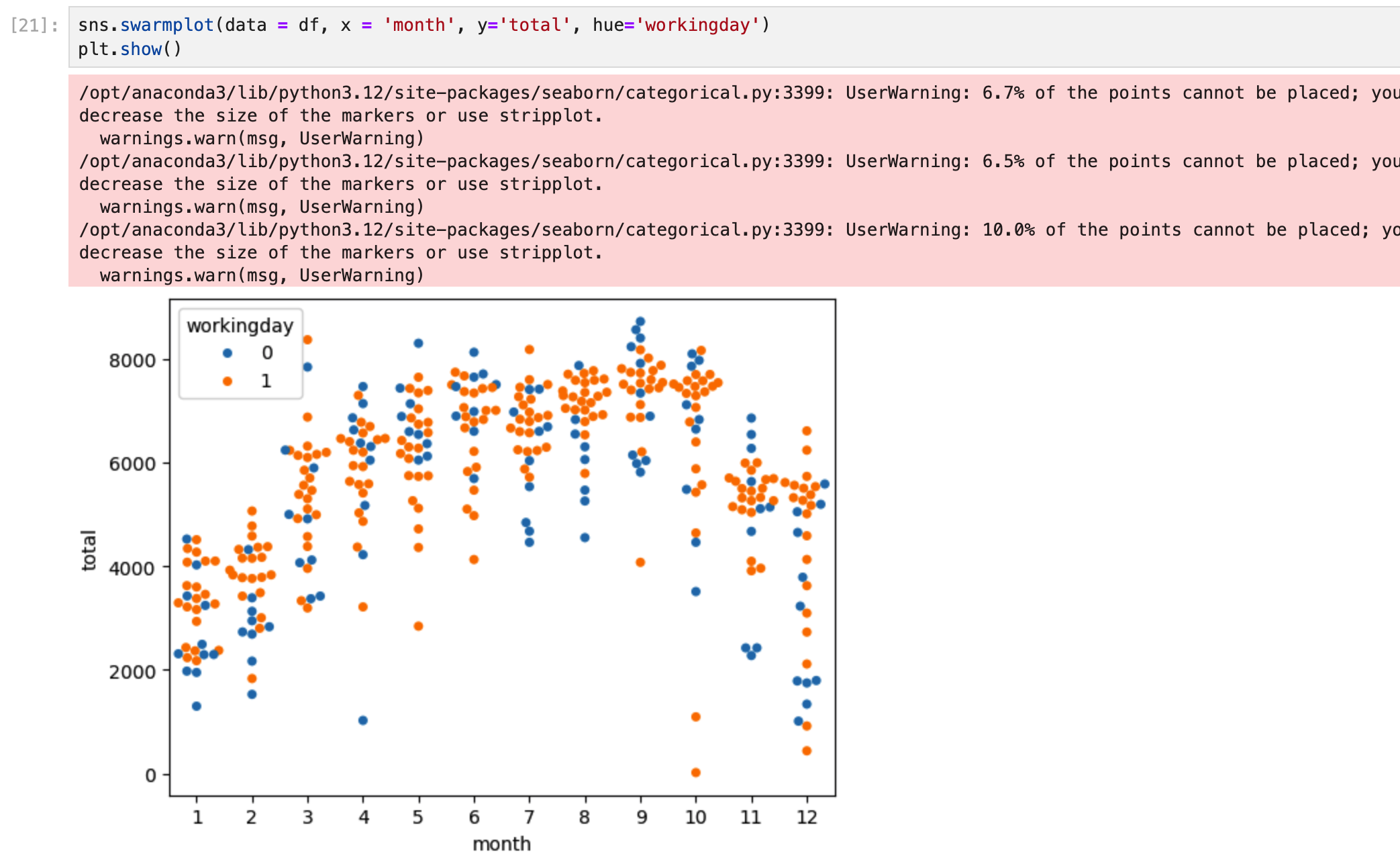
stripplot, swarmplot : 로우가 수십개 ~ 수백개 정도 되는 비교적 작은 데이터셋을 분석할 때 사용
실습
import pandas as pd
import seaborn as sns
import matplotlib.pyplot as plt

bike_df = pd.read_csv('data/bike.csv')
sns.set_theme(rc={'figure.figsize': (10, 5)}, style='white')

# 여기에 코드를 작성하세요.
sns.stripplot(data=bike_df, x='month', y='temperature')
데이터 분포 시각화 2
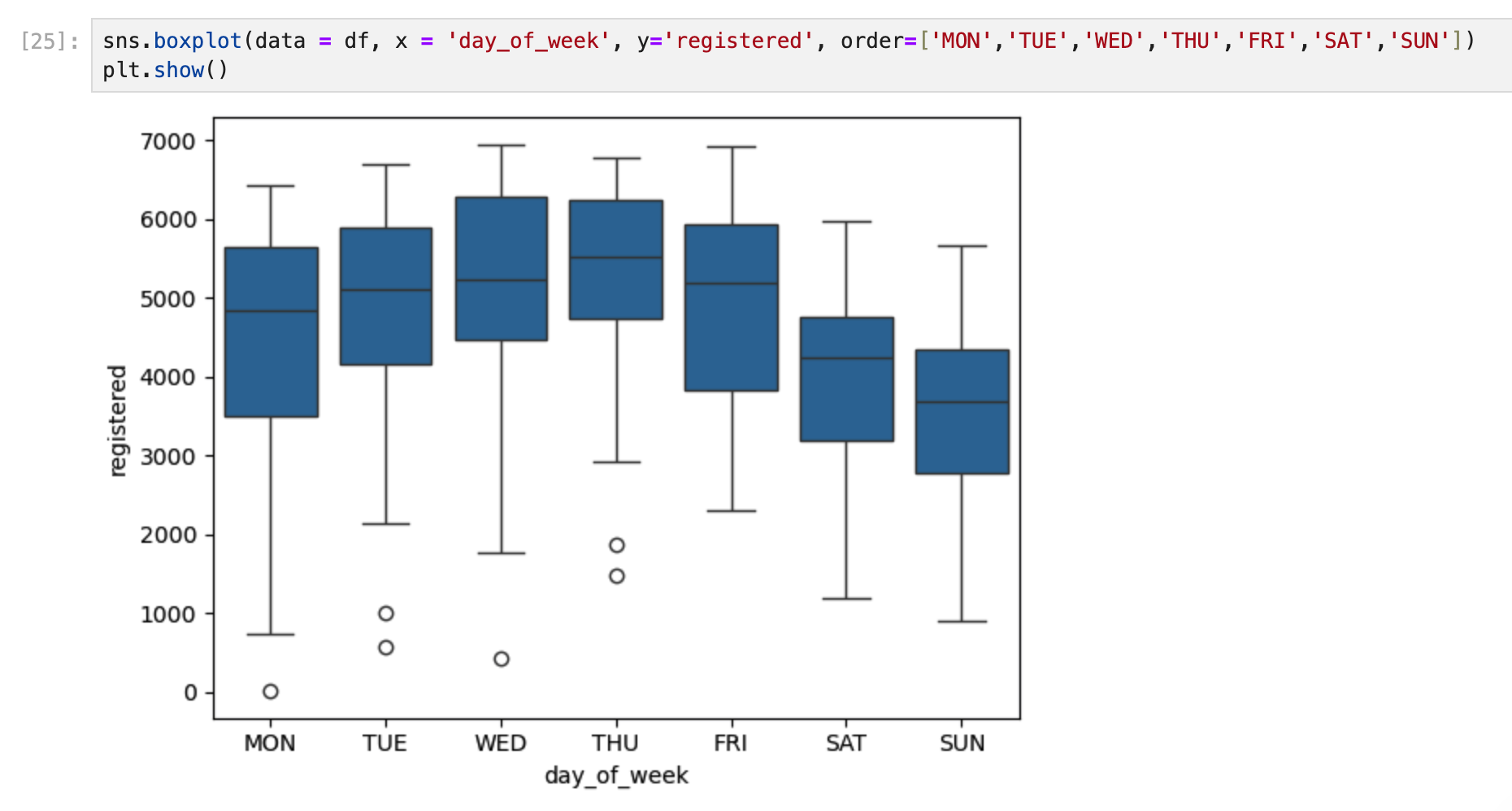
boxplot

order 를 써서 요일을 정렬할 수 있다.
violinplot
박스 플롯과 보는 방식이 거의 유사하다.
흰점이 중간값 두꺼운 막대가 IQR

histplot
한가지 값에 대해 분포를 확인하는 것이므로 x값만 넣음
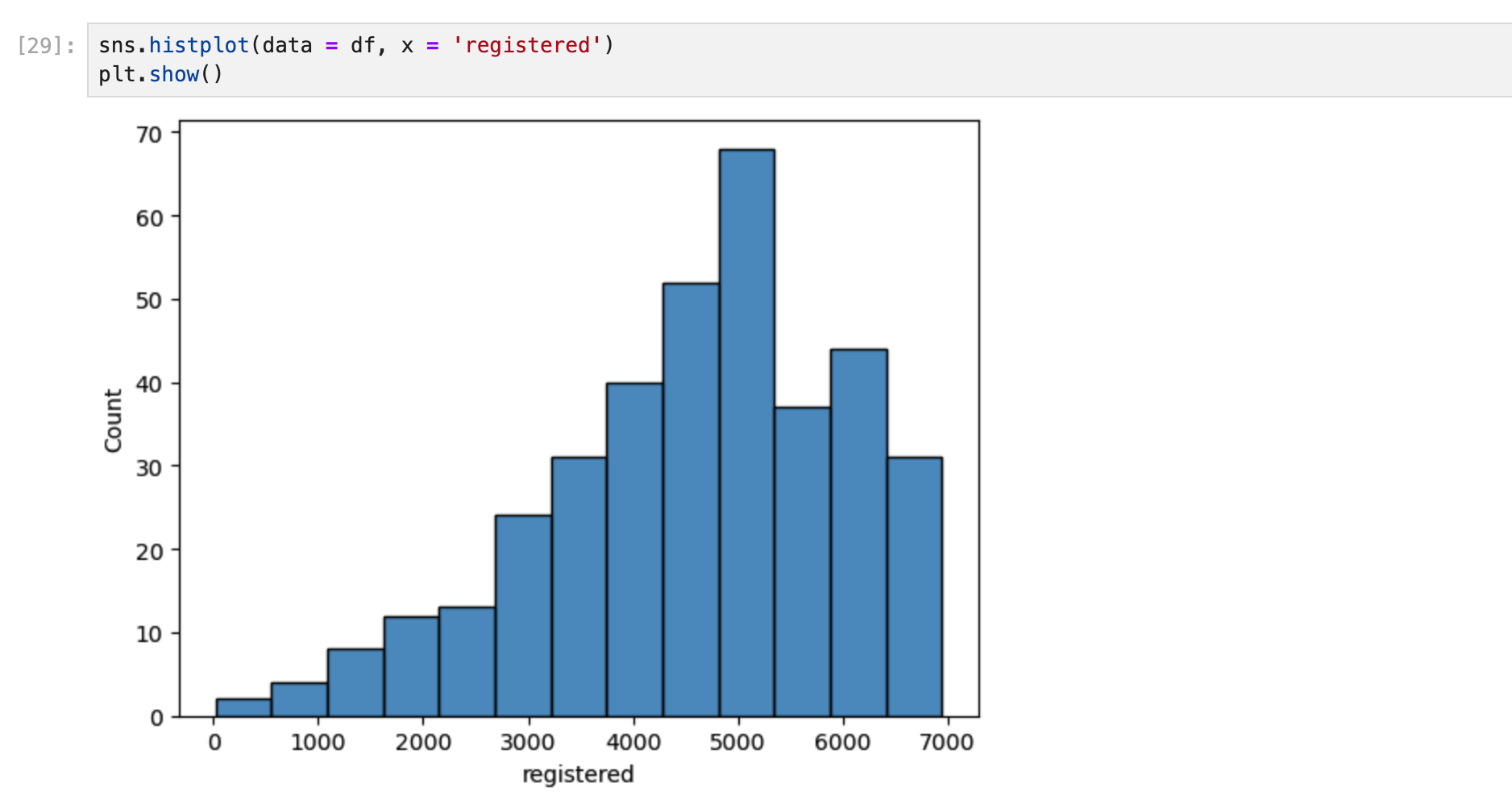
y로 바꾸면 가로로 나옴

multiple을 사용하면 원래 막대그래프에 겹쳐서 나온다.

kdeplot

실습 1
import pandas as pd
import seaborn as sns
import matplotlib.pyplot as plt

flight_df = pd.read_csv('data/flight.csv')
sns.set_theme(rc={'figure.figsize': (6, 6)}, style='white')

# 여기에 코드를 작성하세요.
sns.violinplot(data=flight_df, x='class', y='price')
plt.show()
실습 2
import pandas as pd
import seaborn as sns
import matplotlib.pyplot as plt

insurance_df = pd.read_csv('data/insurance_charge.csv')
sns.set_theme(rc={'figure.figsize': (10, 5)}, style='white')

# 여기에 코드를 작성하세요.
sns.histplot(data=insurance_df, x='charge', hue='smoking', multiple='stack')
plt.show()
상관관계 시각화
산점도
어떤 데이터의 상관관계 확인
상관계수
상관관계를 수로 표현한 것
피어슨 상관계수 (-1 ~ 1)
상관계수 = 0 일때, 두 값 사이에 상관 관계가 없다.
상관계수 > 0 이면, 어떤 값이 커질 때 다른 값도 함께 커진다. (양의 상관관계)
상관계수 < 0 이면, 어떤 값이 커질 때 다른 값은 작아진다. (음의 상관관계)
상관관계의 강도
상관계수가 얼마나 크거나 작은 값인지 확인
값이 1에 가까울수록 강해지고 0에 가까울수록 연관성이 약해진다.
scatterplot

regplot
회귀선 : 가운데 선
두 값의 상관관계를 요약해서 표현하는 역할

이전 그래프에 비해 상관관계가 약해보이고 음의 상관관계 인 것 같다.

상관계수를 확인하는 법

total에 대한 상관계수

상관계수의 값 정렬

색이 진할수록 작은 값, 색이 연할수록 높은 값

실습 1
import pandas as pd
import seaborn as sns
import matplotlib.pyplot as plt

wine_df = pd.read_csv('data/wine.csv')
sns.set_theme(rc={'figure.figsize': (6, 6)}, style='white')

# 여기에 코드를 작성하세요.
sns.regplot(data=wine_df, x='price', y='points')
plt.show()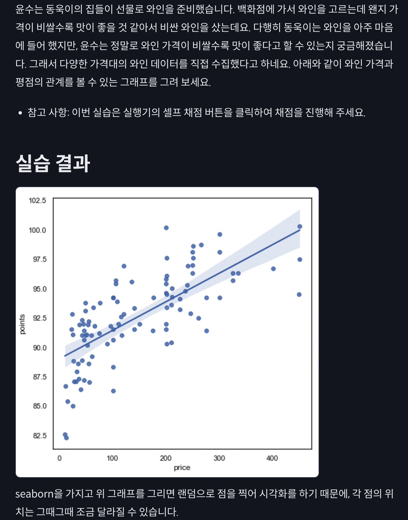
실습 2
import pandas as pd
import seaborn as sns
import matplotlib.pyplot as plt

insurance_df = pd.read_csv('data/insurance_premium.csv')
sns.set_theme(rc={'figure.figsize': (8, 6)}, style='white')

# 여기에 코드를 작성하세요.
sns.heatmap(insurance_df.corr(numeric_only=True),annot=True)
코드잇 12 seaborn
'마케팅 > 데이터 분석' 카테고리의 다른 글
| [파이썬] 데이터 다듬기 (0) | 2025.03.13 |
|---|---|
| [파이썬] DataFrame 기본기 (0) | 2025.03.13 |
| [파이썬] 통계 기본 상식과 그래프 (1) | 2025.03.09 |
| [파이썬] pandas (0) | 2025.02.25 |
| [파이썬] Matplotlib (1) | 2025.02.25 |


